
In recent years, the R language became very popular and its applications are kept increasing its area. The evolution of Big data and Data science created much void for the R developers and language as well. So, this article aims at providing the basics of R programming for beginners, so that they can get started.
Features of R programming
- R is a Free Open-source statistical analytics language.
- The R language has a strong hold of graphical visualization capabilities.
- The R community has grown rapidly and today it is one of the largest active community interms of programming language.
- The programming language has more than 10,000 packages.
- Very useful and powerful for complex statistical and mathematical computations.
- Provides distributed computing systems for faster processing.
- R language is an interpreted languages and does not need any compiler for execution.
- Best fit for Data analysis and Machine learning.
- Supports cross platform and other languages as well.
Basics of R programming
R is way better and beneficial than what we think in this python era. Its computational capabilities are unmatched. This article briefs you on the basics of R programming such as data processing, data analysis, and data visualization.
1. Data processing
The data processing in the R includes multiple methods. Rstudio has many inbuilt datasets that you can use directly. You can also load the data using files and external links.
df<- datasets::airquality
 df
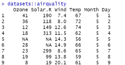
This is the process for loading the data from the in-built data sets. Now we can see how we can import the data using the files.
If you have the CSV file, then you have to execute the below code,
df<- read.csv('sample.csv')
You have to replace the file name in your code. That’s it, your data ready for further analysis. You can also use the “read.table” function in R to red the text data.
2. Data Analysis
R language is particularly made for data analysis and it is no more a secret. So, let’s take a look at the simple data analysis using R programming. You can also see it as the basics of R programming which lets you get started.
Let’s start with reading the data, first and last 10 rows of the data.
head(airquality)
     Ozone Solar.R Wind Temp Month Day
1    41     190    7.4   67     5   1
2    36     118    8.0   72     5   2
3    12     149   12.6   74     5   3
4    18     313   11.5   62     5   4
5    NA      NA   14.3   56     5   5
6    28      NA   14.9   66     5   6
tail(airquality)
      Ozone Solar.R Wind Temp Month Day
148    14      20  16.6   63     9  25
149    30     193   6.9   70     9  26
150    NA     145  13.2   77     9  27
151    14     191  14.3   75     9  28
152    18     131   8.0   76     9  29
153    20     223  11.5   68     9  30
Using the head() and tail() function, you can easily get the top and bottom n rows of the data for the analysis. You can get to know about the data distribution here.
The next will be checking the dimensions of the data. It can be done using the function dim() in R.
dim(airquality)
153 6It returns the output as, the airquality dataset contains 153 rows and 6 columns. These simple functions will save much time in the data analysis.
After this step, we are moving to check the summary of the data using the R function summary(). This function gives you all the information regarding the mean, median, quartiles, min-max values and NA values as well.
summary(airquality)
 Ozone               Solar.R           Wind             Temp           Month

 Min.   :  1.00   Min.   :  7.0   Min.   : 1.700   Min.   :56.00   Min.   :5.000
 1st Qu.: 18.00   1st Qu.:115.8   1st Qu.: 7.400   1st Qu.:72.00   1st Qu.:6.000
 Median : 31.50   Median :205.0   Median : 9.700   Median :79.00   Median :7.000
 Mean   : 42.13   Mean   :185.9   Mean   : 9.958   Mean   :77.88   Mean   :6.993
 3rd Qu.: 63.25   3rd Qu.:258.8   3rd Qu.:11.500   3rd Qu.:85.00   3rd Qu.:8.000
 Max.   :168.00   Max.   :334.0   Max.   :20.700   Max.   :97.00   Max.   :9.000
 NA's   :37       NA's   :7
      Day
 Min.   : 1.0
 1st Qu.: 8.0
 Median :16.0
 Mean   :15.8
 3rd Qu.:23.0
 Max.   :31.0
As you can see here that the summary function returned all the important insights over the input data. What else one can expect from a single function?
The final step in the basics of R programming data analysis is to check for the NA values and replace them with 0.
is.na(df)
       Ozone  Solar.R  Wind  Temp Month   Day
  [1,] FALSE   FALSE FALSE FALSE FALSE FALSE
  [2,] FALSE   FALSE FALSE FALSE FALSE FALSE
  [3,] FALSE   FALSE FALSE FALSE FALSE FALSE
  [4,] FALSE   FALSE FALSE FALSE FALSE FALSE
  [5,]  TRUE    TRUE FALSE FALSE FALSE FALSE
  [6,] FALSE    TRUE FALSE FALSE FALSE FALSE
  [7,] FALSE   FALSE FALSE FALSE FALSE FALSE
  [8,] FALSE   FALSE FALSE FALSE FALSE FALSE
  [9,] FALSE   FALSE FALSE FALSE FALSE FALSE
 [10,]  TRUE   FALSE FALSE FALSE FALSE FALSE
 [11,] FALSE    TRUE FALSE FALSE FALSE FALSE
 [12,] FALSE   FALSE FALSE FALSE FALSE FALSE
wow!!! the is.na function returned the logical values and if there is a NA values it is represented by TRUE value.
df[is.na(df)]<-0
df
      Ozone Solar.R Wind Temp Month Day
1      41     190   7.4   67     5   1
2      36     118   8.0   72     5   2
3      12     149  12.6   74     5   3
4      18     313  11.5   62     5   4
5       0       0  14.3   56     5   5
6      28       0  14.9   66     5   6
7      23     299   8.6   65     5   7
8      19      99  13.8   59     5   8
9       8      19  20.1   61     5   9
10      0     194   8.6   69     5  10
11      7       0   6.9   74     5  11
12     16     256   9.7   69     5  12
As you can see here, all the NA values get replaced by the 0 value. This is how you can check for NA values and negate them using the 0.
3. Data Visualization
The final part of the basics of R programming is visualization. In this section, we are going to plot multiple graphs over the input data and thereby understand the data distribution and behavior.
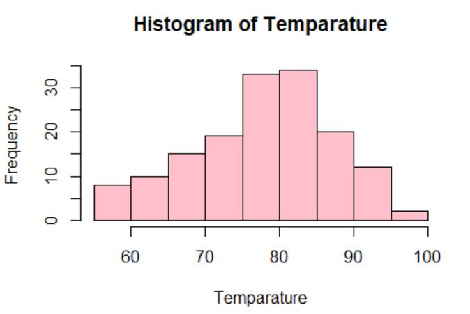
Temparature <- airquality$Temp
hist()
hist(Temparature,col = 'Pink')
Fantastic!
This is the basic histogram plot in the R programming. You can easily pass the data and then plot the histogram using the hist() function I R language.
Wrapping Up – Basics of R programming
R is very useful in data analysis with its impeccable analytical tools and visualization packages.
This article is all about the basics of R programming and I hope it is successful in briefing the same.
That’s all for now. Happy R!!!
More read: R documentation